
|
KeYmaera
or Source |
||

|
Using the KeYmaera Prover for Verifying Hybrid Systems
KeYmaera is a verification tool for hybrid systems and built as a hybrid theorem prover for hybrid systems. KeYmaera separates the overall verification workflow into two phase. In the first phase you specify the hybrid system that you would like to verify along with its correctness properties. In the second phase, you can use KeYmaera and its automatic proof strategies to verify the specified property of the hybrid system.
-
 Load a KeYmaera problem specification using
- Project Assistant with the File->Load Project menu, e.g., for loading Simple Acceleration, or
- Load File to locate a .key problem specification file from your disk with the File->Load menu, e.g., for opening simple.key or use the toolbar
-
 Run the automatic proof strategies to verify your hybrid system with the Proof->Start menu or toolbar.
As a simple example, you can look at the following:
- File->Load Project
- Choose Simple Acceleration example
-
Run the automatic prover with the Proof->Start menu or toolbar
- Depending on your settings, KeYmaera may stop showing you an intermediate result to inspect, just click Proof->Start again to proceed.
- Apply find counterexample rule to see if there is a counterexample for the property, if it cannot be proven.
- Directly select proof rules from the context menu, e.g., to discover parameter constraints for parametric verification.
- Adjust the proof strategy to your needs in the "Hybrid Strategy" tab to tune the proof search procedure of KeYmaera and adapt it to your needs.
- Choose from many computational back-end solvers in "real arithmetic solver" option of the "Hybrid Strategy" tab to customise your prover and tune in to your system environment and improve verification power.
- Select visualization rule to see a graphical view of the transition system. (requirement: install graphviz/dotty)

KeYmaera Problem Specification Files by Example
You can specify the verification problem by loading a .key problem specification file. This file specifies bot the model of your hybrid system (using the notation of hybrid programs) and the correctness property that you want to verify.
Before we introduce the precise syntax of KeYmaera's specification language, we start with two introductory examples.
Example (Controlled Moving Point)
Consider the following simple example of a hybrid controller moving a point
x towards 0 on the real line.
It is a very simple bang-bang controller that pushes x opposite to its sign
such that it moves towards 0.
You can directly ![]() load it in KeYmaera and push the play button
load it in KeYmaera and push the play button ![]() or Proof->Start to prove it automatically.
or Proof->Start to prove it automatically.
\programVariables { /* state variable declarations */ R x; R a; R t, c; } \problem { /* initial state characterization */ x^2 < (4*c)^2 -> \[ /* system dynamics */ ( if (x>0) then a := -4 /* move left */ else a := 4 /* move right */ fi; t := 0; /* reset clock variable t */ {x'=a, t'=1, t<=c} /* continuous evolution */ )* /* repeat these transitions */ \] (x^2 <= (4*c)^2) /* safety / postcondition */ } |
This example contains typical idioms for specifying correctness properties and hybrid systems in KeYmaera:
|
 |
- In the example, the precondition x^2<(4*c)^2 of the implication characterises the set of possible initial states of the system. The controlled moving point system can start in any state satisfying this precondition.
- The hybrid system is specified as a hybrid program within the modality \[...\].
Here, it is given as a controller-plant loop of the canonical form (controller; plant)*.
- The discrete controller adjusts the control choice variable a depending on the current value of x by an if-then-else statement.
- The continuous plant dynamics is specified by a differential equation system x'=a,t'=1 with an additional evolution domain restriction (also confusingly called invariant region) t<=c. This differential equation characterises how the state variables x and t change over time. By the slope of 1, variable t is a clock variable.
- The evolution domain t<=c of the differential equation system specifies that the plant does not leave t<=c, i.e., takes at most c time units, which is a free parameter of the system.
- The overall controller-plant loop repeats any number of times, which is indicated by the * at the end for repetition.
- The postcondition x^2<=(4*c)^2 specifies the safety property that is conjectured to hold for each reachable state.
Example (Bouncing Ball)
| As a standard example, consider the bouncing ball [10]. A ball falls from height h and bounces back from the ground (h=0) after an elastic deformation. The current speed of the ball is denoted by v, and t is a clock measuring the falling time. We assume an arbitrary positive gravity force g and that the ball loses energy according to a damping factor 0≤c<1. |  |
\programVariables {
    /* state variable declarations */
    R h,v,t;
    R c,g,H;
}

\problem {
      /* initial state characterization */
      g>0 & h>=0&t>=0 & 0<=c&c<1 & v^2<=2*g*(H-h) & H>=0
  ->
     \[                          /* system dynamics */
       (
         {h'=v,v'=-g,t'=1, h>=0};/* falling/jumping */
         if (t>0 & h=0) then     /* if on ground */
             v := -c*v;          /* bounce back */
	     t := 0
         fi.
       )*                        /* repeat transitions */
     \] (0<=h & h<=H)            /* safety/postcondition*/
}
The ball loses energy at every bounce, thus the ball never bounces higher than the initial height. This can be expressed by the safety property 0≤h≤H, where H denotes the initial energy level, i.e., the initial height if v=0. The above problem specification states that the ball never bounces higher than that, i.e., it always remains within the region 0≤h≤H when it starts jumping in an appropriate state. For more details on the bouncing ball example, see [10].
Structure of KeYmaera Problem Specification File
A .key input file for KeYmaera specifies both the operational model of your hybrid system (using the notation of hybrid programs) and the correctness property that you want to verify. The verification problem is specified in a block called \problem {...} that contains the problem description as a formula. This block contains a single formula of differential dynamic logic (dL). For instance, this formula can characterise the initial state of the system using implications, the operational system specification using hybrid programs, and the safety/liveness/reactivity/controllability properties to show using modalities.
The .key file format is quite flexible (there is a full description of KeY files with all details except the description of logical formulas in KeYmaera). The canonical case has the following form
\functions {
  /* symbolic parameter declarations */
  /* they cannot change their values at runtime */
  R para1;
  R para2;
}

\programVariables {
    /* state variable declarations */
    R x;
    R y;
    R z;
}

\problem {
    AFormula
}
Here AFormula is a formula in differential dynamic logic (dL) following the syntax of dL formulas. This logical formula specifies the property that you are interested in. It will also include the system dynamics inside modalities following the syntax of hybrid programs. Often (but not always), the formula AFormula has the form
General Philosophy
The general guiding principle behind the notation of hybrid programs is to be able to describe hybrid systems in a language that is a close extension of standard discrete programming languages. Then the discrete parts are easy to implement while the differential equations describe the dynamics of the physical system you want to control. We also want a language that is concise and easy to read, even for more complex systems.
Variables do not just change on their own unless you explicitly tell them to using an assignment x:=t or differential equation like x'=5-a. If you specifically want a variable to change arbitrarily you can use x:=* nondeterministic assignments as needed.
Hybrid Program Syntax for Hybrid Systems
|
In KeYmaera, the behaviour of hybrid systems can be specified easily in a program notation called hybrid programs.
Hybrid programs are a simple program notation for hybrid systems.
Think of taking a standard programming language and adding differential equations in order to be able to talk about the continuous dynamics of the system.
In |
Cheat Sheet and Operators Rules |
| Hybrid programs, with typical names α and β, are a program notation for hybrid systems and are defined by the following syntax | ||
| α ::= | α; β | Sequential composition that runs α first and then β after α stops (β never starts if α never stops) |
| x:=t | Discrete assignment/jump assigning the value of term t to x | |
| x:=* | Nondeterministic assignment assigns any real value to x, non-deterministically | |
| ?H | State assertion testing whether formula H is true in current state (otherwise abort) | |
| α ++ β | Non-deterministic choice following either alternative α or β | |
| α* | Non-deterministic repetition, repeating α arbitrarily often including 0 times | |
| {x'=t,y'=s, H} | Continuous evolution along differential equation system with terms t,s, optionally with evolution domain constraint H. This domain constraint H needs to be true at every time during the evolution, otherwise the system needs to stop following this continuous mode and move on. You can use systems of differential equations, differential-algebraic equations, differential inequalities, and differential equations with disturbances. | |
| if(H) then α fi | If-then statement, performs α if formula/condition H holds at current state and does nothing otherwise | |
| if(H) then α else β fi | If-then-else statement, performs α if H holds at current state and performs β otherwise | |
| while(H) α end | While loop, repeats α as long as H holds, stops before doing α only if H is false (α will not be stopped in the middle just because H becomes false at some intermediate state during α). | |
| {x'=t,y'<=s,y'>=r, H} | Continuous evolution along system of differential equations and differential inequalities with terms t,s,r, optionally with evolution domain H. The time-derivative of y needs to stay within r and s all the time. Hybrid programs with differential inequalities are called differential-algebraic programs. | |
| {\exists R d . (x'=t & y'=s & H)} | Continuous evolution along system of differential-algebraic equations with disturbance d (which may occur in the terms t,s and formula H), optionally with evolution domain H. Hybrid programs with differential-algebraic constraints are called differential-algebraic programs. | |
| R x | Variable declaration, declaring x as a real variable (either a state variable or auxiliary variable). | |
| R x, y, z | Variable declaration, declaring x, y, and z as real variables | |
| where H is a formula of (possibly non-linear) real arithmetic (possibly including quantifiers, but no modalities). | ||
| Quantified hybrid programs, with typical names α and β, are a program notation for distributed hybrid systems and are defined by the extending the above syntax for hybrid programs with the following cases | ||
| \forall C i . x(i):=t(i) | Quantified discrete assignment assigning the values of the terms t(i) to the x(i) for all i of type C. | |
| \forall C i . x(i):=* | Quantified nondeterministic assignment assigning any value to the x(i) for all i of type C. The values are chosen nondeterministically and independently for each i. | |
| \forall C i . {x(i)'=t(i), y(i)'=s(i), H(i)} | Quantified continuous evolution along quantified differential equation system evolving x(i) and y(i) simultaneously with rates described by terms t(i),s(i) for all i of type C, optionally with evolution domain constraint H(i). This domain constraint H(i) needs to be true for all i at every time during the evolution, otherwise the system needs to stop following this continuous mode and move on. | |
Formula Syntax for Properties of Hybrid Systems
|
In KeYmaera, the safety/liveness/reactivity/controllability properties that you are interested in can be specified using formulas of differential dynamic logic.
In these formulas, the actual hybrid system to consider can be embedded easily as a hybrid program.
In |
Cheat Sheet and Operators Rules |
| Formulas of differential dynamic logic dL, with typical names φ and ψ, are defined by the following syntax | ||
| φ ::= | !φ | Negation (not) |
| φ & ψ | Conjunction (and) | |
| φ | ψ | Disjunction (or) | |
| φ -> ψ | Implication (implication) | |
| φ <-> ψ | Biimplication (equivalence) | |
| \forall R x . φ | Universal quantifier: for all real values for variable x, formula φ holds | |
| \exists R x . φ | Existential quantifier: for some real value for variable x, formula φ holds | |
| \[α\] φ | Box-modality: After all runs of hybrid program α, formula φ holds (safety) | |
| \<α\> φ | Diamond-modality: There is at least one run of hybrid program α, after which formula φ holds (liveness) | |
| \[[α\]] φ | Temporal-box-modality: During all runs of hybrid program α, formula φ holds (safety throughout) | |
| pred | Real arithmetic predicate expression | |
| Formulas of quantified differential dynamic logic QdL, with typical names φ and ψ, are defined by the same syntax as dL except that α can be a quantified hybrid program in the modalities and that multiple sorts other than the reals R can be used: | ||
| \forall C x . φ | Universal quantifier: for all values of type C for variable x, formula φ holds | |
| \exists C x . φ | Existential quantifier: for some value of type C for variable x, formula φ holds | |
| \[α\] φ | Box-modality: After all runs of quantified hybrid program α, formula φ holds (safety) | |
| \<α\> φ | Diamond-modality: There is at least one run of quantified hybrid program α, after which formula φ holds (liveness) | |
| Real arithmetic predicate expressions are defined by the following syntax | ||
| pred ::= | t > s | Greater than |
| t >= s | Greater equals | |
| t = s | Equals | |
| t != s | Not equal | |
| t <= s | Less equals | |
| t < s | Less than | |
| Real arithmetic terms, with typical names s and t, are defined by the following syntax | ||
| t ::= | t + s | Addition |
| t - s | Subtraction | |
| t * s | Multiplication | |
| t / s | Division | |
| t^n | Power with integer n | |
| - s | Minus | |
| f(t1,...,tn) | Function application | |
| VARIABLE | An arbitrary variable identifier (that has been declared) | |
| NUMBER | An arbitrary decimal number | |
@Annotations for Verification
In order to help KeYmaera find proofs, you can use user interaction or annotate your problem. Both can be quite powerful for proving advanced properties and properties of complex systems that KeYmaera cannot yet prove fully automatically on its own or where it simply takes too long for KeYmaera to find a proof.
To help KeYmaera, you can annotate your problem using @invariant and @candidate annotations.
- @invariant(F)
- When used as α*@invariant(F), the annotation annotates loop α with a recommendation to use the formula F as a loop invariant for the loop induction proof rule ind loop invariant. When used as {x'=y,y'=s, H}@invariant(F), the annotation annotates the differential equation system with differential invariant F for the proof.
- @invariant(F1,F2,F3,...,Fn)
- When used as {x'=y,y'=s, H}@invariant(F1,F2,F3,...,Fn), the annotation annotates the differential equation system with differential invariants for the proof (using differential cuts). KeYmaera will first use a differential cut by formula F1. If this differential invariant succeeds, KeYmaera will use a differential cut by formula F2 and so on. Finally, KeYmaera will try to prove the original property using all the auxiliary information that has accumulated in differential cuts, see [6,9,11] for details on this process and its automation.
- @variant($n,F)
- When used as α*@variant($n,F), the annotation annotates loop α with a recommendation to use the formula F as a loop variant for the loop induction proof rule con loop convergence, where $n is the variable measuring progress, which usually occurs in F.
- @candidate(F1,F2,F3,...,Fn)
- The @candidate(F1,F2,F3,...,Fn) annotation works like the @invariant annotation, except that it only suggests interesting candidates for proof search that KeYmaera can try. KeYmaera will keep on trying also other options and is not fully committed to these choices. This can be very useful for searching and playing with different proof options.
The following example, which happens to be a simple circular aircraft maneuver, illustrates annotations for invariants for loops and differential invariants for differential equations. They are actually not necessary, because KeYmaera finds the proof automatically without annotations. But it is a good illustration of annotations that enable KeYmaera to find a proof quicker. They are also good comments explaining why the system works correctly.
\functions {
  R protectedzone;
}

\programVariables {
  /* aircraft at position (x1,x2) in direction (d1,d2) */
  R x1,x2, d1,d2;
  /* aircraft at position (y1,y2) in direction (e1,e2) */
  R y1,y2, e1,e2;
  /* angular velocities and center */
  R om, omy, c1,c2;
}

\problem {
    (x1-y1)^2 + (x2-y2)^2 >= protectedzone^2
->
 \[(
   (
    om:=*;omy:=*;
    {x1'=d1,x2'=d2, d1'=-om*d2,d2'=om*d1,
     y1'=e1,y2'=e2, e1'=-omy*e2,e2'=omy*e1,
     ((x1-y1)^2 + (x2-y2)^2 >= protectedzone^2)}
   )*@invariant((x1-y1)^2+(x2-y2)^2 >= protectedzone^2);
   c1:=*;c2:=*; om:=*;
   d1:=-om*(x2-c2); d2:=om*(x1-c1);
   e1:=-om*(y2-c2); e2:=om*(y1-c1);
   {x1'=d1,x2'=d2, d1'=-om*d2,d2'=om*d1,
    y1'=e1,y2'=e2, e1'=-om*e2,e2'=om*e1}
    @invariant(d1-e1=-om*(x2-y2)&d2-e2=om*(x1-y1))
  )*@invariant((x1-y1)^2 + (x2-y2)^2 >= protectedzone^2)
 \] ( (x1-y1)^2 + (x2-y2)^2 >= protectedzone^2 )
}
KeYmaera provides some additional annotations for more fine-grained control, but you will not need them very often.
- @weaken
- The @weaken annotation instructs KeYmaera to try to weaken the differential equation that it annotates. This annotation is rarely necessary, but can still speed up some proof search or cut down lengthy computations.
The following example is a variation of the annotations from above, with an explicit @weaken. The annotations are not necessary, because KeYmaera finds the proof automatically without annotations.
\functions {
  R protectedzone;
}

\programVariables {
  /* aircraft at position (x1,x2) in direction (d1,d2) */
  R x1,x2, d1,d2;
  /* aircraft at position (y1,y2) in direction (e1,e2) */
  R y1,y2, e1,e2;
  /* angular velocities and center */
  R om, omy, c1,c2;
}

\problem {
    (x1-y1)^2 + (x2-y2)^2 >= protectedzone^2
->
 \[(
   (
    om:=*;omy:=*;
    {x1'=d1,x2'=d2, d1'=-om*d2,d2'=om*d1,
     y1'=e1,y2'=e2, e1'=-omy*e2,e2'=omy*e1,
     ((x1-y1)^2 + (x2-y2)^2 >= protectedzone^2)}@weaken()
   )*@invariant((x1-y1)^2+(x2-y2)^2 >= protectedzone^2);
   c1:=*;c2:=*; om:=*;
   d1:=-om*(x2-c2); d2:=om*(x1-c1);
   e1:=-om*(y2-c2); e2:=om*(y1-c1);
   {x1'=d1,x2'=d2, d1'=-om*d2,d2'=om*d1,
    y1'=e1,y2'=e2, e1'=-om*e2,e2'=om*e1}
    @invariant(d1-e1=-om*(x2-y2)&d2-e2=om*(x1-y1))
  )*@invariant((x1-y1)^2 + (x2-y2)^2 >= protectedzone^2)
 \] ( (x1-y1)^2 + (x2-y2)^2 >= protectedzone^2 )
}
In this keymaera file, the green @annotations are non-operational, but useful proof hints. They do not change what the system does or what the property means. Annotations only affect proof search, not meaning. In particular, consider the differential equation block
In the above keymaera file, when stripping out all the green @annotations, the problem still means the same thing and it can still be proved. It just takes KeYmaera a little longer. In more complex systems, however, annotations can be really useful.
The transition system of the above example looks as follows

Additional Function Symbols
Most of the time, you won't need additional function symbols. But in case you do, here's how. Before the \problem-block of a problem specification file, you can declare auxiliary functions that you intend to use in the system specification. This block is called \functions {...} and contains definitions of function symbols used in the system specification. The functions are declared using their return type, name and argument types. Use, e.g., R f(R,R); to declare a function f of type reals with two real-valued arguments. Or use R c; to declare a real-valued constant function with no arguments.
\functions {
  /* symbolic parameter declarations */
  /* they cannot change their values at runtime */
  R c;
  R mindistance;
  /* function symbol declarations */
  /* they cannot change their values at runtime */
  R f(R,R);
  R g(R);
}
Note that these are logical function symbols.
In a nutshell, program variables declared inside hybrid programs are state variables that can change their value during system execution. Symbols and functions declared in the \functions block are constant symbols, i.e., cannot change their value during system execution.
For details concerning the distinction of rigid logical function symbols compared to flexible state variables declared in hybrid programs, see book, sections 2.2.1 and 2.3.1.
More advanced function declarations are possible as well, including \external functions that are to be interpreted by the arithmetic backend, and \nonRigid function symbols that can be assigned to in quantified differential dynamic logic.
\functions {
  /* symbolic parameter declarations */
  /* they cannot change their values at runtime */
  R para1;
  R para2;
  /* declare a function as external, i.e., */
  /* to be interpreted by the arithmetic backend */
  \external R Sqrt(R);
  /* Only in quantified differential dynamic logic QdL */
  /* declare an assignable function with 3 parameters */
  \nonRigid[Location] R f(C,C,D);
}
Note that when declaring \external functions (like Sqrt, Abs, Log, Sin, Cos), you need to make sure that the arithmetic backend you are working with actually understands them as expected.
Representing Hybrid Automata as Hybrid Programs
In much the same way as finite automata can be written as programs or timed automata can be represented as real-time programs, Hybrid automata can be represented naturally as hybrid programs. Hybrid programs essentially correspond to a program rendition of hybrid automata.
The following simple example corresponds to a water tank, which regulates water level y between 1 and 12 by filling or emptying the water tank.
 |
 |
/* This example does NOT use a good description style */
\programVariables {
    /* state variable declarations */
    R y, x, st;
}

\problem {
    /* initialization */
    \[  x:=0; y:=1; st:=0 \] (
     st = 0  /* initial state characterization */
   ->
     \[  /* system dynamics */
       ( /* repeat the discrete/continuous transitions */
           (?(st=0);
                 (?(y=10); x:=0; st:=1)
              ++ {x'=1,y'=1, y<=10}
           )
        ++ (?(st=1);
                 (?(x=2); st:=2)
              ++ {x'=1,y'=1, x<=2}
           )
        ++ (?(st=2);
                 (?(y=5); x:=0; st:=3)
              ++ {x'=1,y'=-2, y>=5}
            )
        ++ (?(st=3);
                 (?(x=2); st:=0)
              ++ {x'=1,y'=-2, x<=2}
           )
      )*@invariant(1<=y & y<=12
           & (st=3 -> (y>=5-2*x)) & (st=1 -> (y<=10+x)))
     \] (1<=y & y<=12)    /* safety / postcondition */
   )
  }
Note that this automaton style is generally a bad choice for describing your system model. Look at the @invariant-annotation for the weird state encodings. This is not a good system model. Be advised that we encourage the development of systems directly in terms of hybrid programs, not translate them from automata. This exploits the notational power and often gives much more natural system descriptions than formal translation. The improved representational power of hybrid programs also helps making verification more scalable.
When you want to avoid encoding state/mode information as numbers, you can also use the following pattern to declare mnemonic constants (essentially as an enum):/* This example does NOT use a good description style */ \programVariables { /* state variable declarations */ R y, x, st; /* mode variables */ R fill, stop, drain, start; } \problem { /* initialization */ \[ x:=0; y:=1; fill:=0; stop:=1; drain:=2; start:=3; st:=fill \] ( st = fill /* initial state characterization */ -> \[ /* system dynamics */ ( /* repeat the discrete/continuous transitions */ (?(st=fill); (?(y=10); x:=0; st:=stop) ++ {x'=1,y'=1, y<=10} ) ++ (?(st=stop); (?(x=2); st:=drain) ++ {x'=1,y'=1, x<=2} ) ++ (?(st=drain); (?(y=5); x:=0; st:=start) ++ {x'=1,y'=-2, y>=5} ) ++ (?(st=start); (?(x=2); st:=fill) ++ {x'=1,y'=-2, x<=2} ) )*@invariant(1<=y & y<=12 & (st=start->(y>=5-2*x)) & (st=stop->(y<=10+x))) \] (1<=y & y<=12) /* safety / postcondition */ ) }
All hybrid automata can be represented easily as hybrid programs using a construction that is very similar to the construction that implements finite automata as programs. Note, however, that the quality of the hybrid program can sometimes be better if the system is designed as a hybrid program right away, instead of being converted. We generally recommend starting with hybrid programs in the first place.
KeYmaera Prover Usage, Verification, and Automation
For proving the specified properties of the hybrid system run KeYmaera,
load the problem specification file and press the play button ![]() or the Proof->Start menu to verify it.
In addition, you can apply the Find Counterexample rule to find if there is a counterexample for the property and display it.
Furthermore, you can select proof rules from the context menu in case the automatic strategy stops.
or the Proof->Start menu to verify it.
In addition, you can apply the Find Counterexample rule to find if there is a counterexample for the property and display it.
Furthermore, you can select proof rules from the context menu in case the automatic strategy stops.
If you want KeYmaera to prove your examples automatically, select
auto for the Differential Saturation option in the
Hybrid Strategy tab before you click on ![]() start prover.
start prover.
If you prefer to work more interactively, select off instead, which can help you understand the working principle of KeYmaera better. When you run the prover with Differential Saturation switched off, KeYmaera will stop and ask you which way to go when it is unsure. Turning the automatic Differential Saturation procedure off or selecting simple can also help you verify examples that are beyond the capabilities of today's arithmetic solvers.
User Interactions for Verification
KeYmaera has a number of powerful proof strategies and can be tuned to perform even better by configuring various options. Nevertheless, for learning purposes, for experimenting with and exploring different system designs, and for helping KeYmaera to find proofs, it can be really useful to apply proof rules manually. In order to help KeYmaera find proofs, you can use user interaction or annotate your problem. Both can be quite powerful for proving advanced properties and properties of complex systems that KeYmaera cannot yet prove on its own or where it takes too long.
KeYmaera has a very powerful user interface that gives the user a lot of possibilities and flexibility in how he wants to conduct his system verification. For user interaction, you can just apply some proof rules manually by right-clicking on subformulas/ It can also be useful to hit Proof->Start, then, after some time, use Proof->Stop, and look at the outcome to see where the KeYmaera prover went and take it from there. If KeYmaera went the wrong way on some of the branches, you can also just use Proof->Goal Back or Proof->Prune Proof to go back and try a different way.
Also see FAQ How to apply proof rule and FAQ How to use goal back.
Prover Settings and Arithmetic
KeYmaera supports several different settings and real arithmetic procedures. You have multiple options to choose from in the real arithmetic solver options of the Hybrid Strategy tab. You can also control using built-in arithmetic and built-in inequalities if you want to enable internal handling of arithmetic or use the back-end arithmetic directly.
Depending on the number of tools you have configured, you have several options for handling real arithmetic to choose from:
- Built-in Gröbner Bases and Fourier-Motzkin arithmetic [12]
- Mathematica
- Z3 SMT Solver by Microsoft Research
- Reduce/Redlog (if you compile it, use CSL lisp)
- QEPCAD B or QEPCAD B for Mac
- Built-in Cohen-Hörmander Quantifier Elimination by David Renshaw
- HOL Light
- Cohen-Hörmander Quantifier Elimination
- Gröbner Bases (built-in)
- Semi-definite Programming for the Positivstellensatz using CSDP
- Semi-definite Programming for the Real Nullstellensatz [12] using CSDP
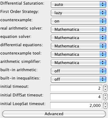
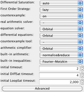
Other settings can be useful too, e.g., choosing IBC as the choice for the First Order Strategy.
More Information
The single most comprehensive source on background material and more information about KeYmaera and its underlying verification approach is the book Logical Analysis of Hybrid Systems: Proving Theorems for Complex Dynamics [17]. The canonical references on the KeYmaera approach are [5,6,25].
To get a first impression, you can also look at the LICS'12 tutorial slides or CAV'11 tutorial slides, the slides for differential dynamic logic, the KeYmaera Tool Paper, related publications. The various publications about KeYmaera case studies [15,13,16,14,20,21,22] can be useful to understand how complicated systems and complicated properties can be verified with KeYmaera. There is A Short Introduction to Using KeYmaera. Answers to typical questions can be found in the KeYmaera FAQ.
If you are interested in understanding more of the internal working principles of the underlying KeY system, you can also read the KeY-Book, or the KeY tutorials. See full description of KeY files and description of logical formulas in KeYmaera.
Selected Publications
-
André Platzer.
Dynamic logics of dynamical systems.
arXiv:1205.4788, May 2012. Long version of LICS'12 invited tutorial.
[bib | ⧉ | pdf | arXiv | LICS'12 | abstract]
-
André Platzer.
A differential operator approach to equational differential invariants.
In Lennart Beringer and Amy Felty, editors, Interactive Theorem Proving, International Conference, ITP 2012, August 13-15, Princeton, USA, Proceedings, volume 7406 of LNCS, pp. 28-48. Springer, 2012. © Springer
Invited paper.
[bib | ⧉ | pdf | doi | slides | abstract]
-
André Platzer.
Logics of dynamical systems.
ACM/IEEE Symposium on Logic in Computer Science, LICS 2012, June 25–28, 2012, Dubrovnik, Croatia, pp. 13-24. IEEE 2012. © IEEE
Invited paper.
[bib | ⧉ | pdf | doi | slides | abstract]
-
André Platzer.
The complete proof theory of hybrid systems.
ACM/IEEE Symposium on Logic in Computer Science, LICS 2012, June 25–28, 2012, Dubrovnik, Croatia, pp. 541-550. IEEE 2012. © IEEE
[bib | ⧉ | pdf | doi | slides | TR | abstract]
-
André Platzer.
The structure of differential invariants and differential cut elimination.
Logical Methods in Computer Science 8(4), pp. 1-38, 2012. © The author
[bib | ⧉ | pdf | doi | mypdf | arXiv | abstract]
-
André Platzer.
A complete axiomatization of quantified differential dynamic logic for distributed hybrid systems.
Logical Methods in Computer Science 8(4), pp. 1-44, 2012.
Special issue for selected papers from CSL'10. © The author
[bib | ⧉ | pdf | doi | mypdf | arXiv | CSL'10 | abstract]
-
Stefan Mitsch, Sarah M. Loos and André Platzer.
Towards formal verification of freeway traffic control.
In Chenyang Lu, editor, ACM/IEEE Third International Conference on Cyber-Physical Systems ICCPS'12, Beijing, China, April 17-19. pp. 171-180, IEEE. 2012. © IEEE
[bib | ⧉ | pdf | doi | slides | study | abstract]
-
Sarah M. Loos and André Platzer.
Safe intersections: At the crossing of hybrid systems and verification.
In Kyongsu Yi, editor, 14th International IEEE Conference on Intelligent Transportation Systems, ITSC'11, Washington, DC, USA, Proceedings, pp. 1181-1186. 2011. © IEEE
[bib | ⧉ | pdf | doi | slides | study | abstract]
-
Sarah M. Loos, André Platzer and Ligia Nistor.
Adaptive cruise control:
Hybrid, distributed, and now formally verified.
In Michael Butler and Wolfram Schulte, editors, 17th International Symposium on Formal Methods, FM, Limerick, Ireland, Proceedings, volume 6664 of LNCS, pp. 42-56. Springer, 2011. © Springer
[bib | ⧉ | pdf | doi | slides | study | TR | abstract]
-
André Platzer.
Logic and compositional verification of hybrid systems.
In Ganesh Gopalakrishnan and Shaz Qadeer, editors, Computer Aided Verification, CAV 2011, Snowbird, UT, USA, Proceedings, volume 6806 of LNCS, pp. 28-43. Springer, 2011. © Springer
Invited tutorial.
[bib | ⧉ | pdf | doi | slides | abstract]
-
André Platzer.
Quantified differential dynamic logic for distributed hybrid systems.
In Anuj Dawar and Helmut Veith, editors, Computer Science Logic, 19th EACSL Annual Conference, CSL 2010, Brno, Czech Republic, August 23-27, 2010. Proceedings, volume 6247 of LNCS, pp. 469-483. Springer, 2010. © Springer
[bib | ⧉ | pdf | doi | slides | TR | LMCS'12 | abstract]
-
André Platzer.
Logical Analysis of Hybrid Systems:
Proving Theorems for Complex Dynamics.
Springer, Heidelberg, 2010. 426 pages. ISBN 978-3-642-14508-7.
[bib | ⧉ | doi | book | web | errata | abstract]
-
André Platzer and Jan-David Quesel.
European Train Control System: A Case Study in Formal Verification.
Reports of SFB/TR 14 AVACS 54, 2009. ISSN: 1860-9821, www.avacs.org.
[bib | ⧉ | pdf | ICFEM'09]
-
André Platzer and Jan-David Quesel.
European Train Control System: A case study in formal verification.
In Karin Breitman and Ana Cavalcanti, editors, 11th International Conference on Formal Engineering Methods, ICFEM'09, Rio de Janeiro, Brasil, Proceedings, volume 5885 of LNCS, pp. 246-265. Springer, 2009. © Springer
[bib | ⧉ | pdf | doi | slides | kyx | TR | old | abstract]
-
André Platzer and Edmund M. Clarke.
Formal Verification of Curved Flight Collision Avoidance Maneuvers: A Case Study.
School of Computer Science, Carnegie Mellon University, CMU-CS-09-147, 2009.
[bib | ⧉ | pdf | FM'09]
-
André Platzer and Edmund M. Clarke.
Formal verification of curved flight collision avoidance maneuvers: A case study.
In Ana Cavalcanti and Dennis Dams, editors, 16th International Symposium on Formal Methods, FM, Eindhoven, Netherlands, Proceedings, volume 5850 of LNCS, pp. 547-562. Springer, 2009. © Springer
FM Best Paper Award.
[bib | ⧉ | pdf | doi | slides | study | TR | abstract]
-
André Platzer, Jan-David Quesel and Philipp Rümmer.
Real world verification.
In Renate A. Schmidt, editor, International Conference on Automated Deduction, CADE-22, Montreal, Canada, Proceedings, volume 5663 of LNCS, pp. 485-501. Springer, 2009. © Springer
[bib | ⧉ | pdf | doi | slides | study | TR | smtlib | abstract]
Introduces a decision procedure for universal nonlinear real arithmetic combining Gröbner bases and semidefinite programming for the Real Nullstellensatz.
-
André Platzer and Edmund M. Clarke.
Computing differential invariants of hybrid systems as fixedpoints.
Formal Methods in System Design 35(1), pp. 98-120, 2009.
Special issue for selected papers from CAV'08. © Springer
[bib | ⧉ | pdf | doi | study | CAV'08 | abstract]
-
André Platzer and Jan-David Quesel.
KeYmaera: A hybrid theorem prover for hybrid systems.
In Alessandro Armando, Peter Baumgartner and Gilles Dowek, editors, Automated Reasoning, Fourth International Joint Conference, IJCAR 2008, Sydney, Australia, Proceedings, volume 5195 of LNCS, pp. 171-178. Springer, 2008. © Springer
[bib | ⧉ | pdf | doi | slides | tool | abstract]
-
André Platzer and Edmund M. Clarke.
Computing differential invariants of hybrid systems as fixedpoints.
In Aarti Gupta and Sharad Malik, editors, Computer Aided Verification, CAV 2008, Princeton, USA, Proceedings, volume 5123 of LNCS, pp. 176-189, Springer, 2008. © Springer
[bib | ⧉ | pdf | doi | slides | study | TR | FMSD'09 | abstract]
-
André Platzer and Edmund M. Clarke.
Computing Differential Invariants of Hybrid Systems as Fixedpoints.
School of Computer Science, Carnegie Mellon University, CMU-CS-08-103, Feb, 2008.
[bib | ⧉ | pdf | CAV'08]
-
André Platzer and Jan-David Quesel.
Logical verification and systematic parametric analysis in train control.
In Magnus Egerstedt and Bud Mishra, editors, Hybrid Systems: Computation and Control, 11th International Conference, HSCC 2008, St. Louis, USA, Proceedings, volume 4981 of LNCS, pp. 646-649. Springer, 2008. © Springer
[bib | ⧉ | pdf | doi | poster | abstract]
-
André Platzer.
Differential-algebraic dynamic logic for differential-algebraic programs.
Journal of Logic and Computation 20(1), pp. 309-352, 2010.
Special issue for selected papers from TABLEAUX'07. © The author
[bib | ⧉ | pdf | doi | eprint | study | errata | TABLEAUX'07 | abstract]
-
André Platzer.
Differential dynamic logic for hybrid systems.
Journal of Automated Reasoning 41(2), pp. 143-189, 2008. © The author
[bib | ⧉ | pdf | doi | mypdf | study | abstract]
-
André Platzer.
Combining deduction and algebraic constraints for hybrid system analysis.
In Bernhard Beckert, editor, 4th International Verification Workshop, VERIFY'07, Bremen, Germany, CEUR Workshop Proceedings, 259:164-178, 2007.
[bib | ⧉ | pdf | eprint | slides | abstract]
-
André Platzer.
Differential dynamic logic for verifying parametric hybrid systems.
In Nicola Olivetti, editor, Automated Reasoning with Analytic Tableaux and Related Methods, International Conference, TABLEAUX 2007, Aix en Provence, France, July 3-6, 2007, Proceedings, volume 4548 of LNCS, pp. 216-232. Springer, 2007. © Springer
TABLEAUX Best Paper Award.
[bib | ⧉ | pdf | doi | slides | study | TR | abstract]
-
André Platzer.
A temporal dynamic logic for verifying hybrid system invariants.
In Sergei Artemov and Anil Nerode, editors, Logical Foundations of Computer Science, International Symposium, LFCS 2007, New York, USA, Proceedings, volume 4514 of LNCS, pp. 457-471. Springer, 2007. © Springer
[bib | ⧉ | pdf | doi | slides | study | TR | abstract]
-
André Platzer.
Differential logic for reasoning about hybrid systems.
In Alberto Bemporad, Antonio Bicchi and Giorgio Buttazzo, editors, Hybrid Systems: Computation and Control, 10th International Conference, HSCC 2007, Pisa, Italy, Proceedings, volume 4416 of LNCS, pp. 746-749. Springer, 2007. © Springer
[bib | ⧉ | pdf | doi | poster | abstract]